Most of this site is about AI workflows. This piece is deliberately not, because the point of Krylov is to reach for whatever the problem actually needs, and a lot of engineering problems are still best answered with classical numerics. Here is one worked all the way through.
Welding with a laser is a delicate process up close. A tightly focused beam sweeps along a seam and melts a small pool of metal, often no bigger than a grain of rice, that travels with it. Inside that pool the molten metal swirls, dragged around by differences in surface tension; heat races ahead of the beam and trails behind it in a long wake; and once everything cools and freezes, the part is left slightly distorted. Each of these changes the others, so to predict a weld you have to follow all of them at once.
One coupled model
I built the whole picture as a single coupled finite-element model: fluid flow in the melt, heat transport through the plate, and the solidification that ties them together, solved as one system rather than three loosely linked simulations. It runs in jNO, a small weak-form finite-element library I work on, where the code ends up reading like the equations themselves: each term of the system is one line.
None of that is machine learning. It is Navier–Stokes coupled to heat transport, discretised with Taylor–Hood elements, marched in time with backward Euler, and solved at each step with Newton’s method, textbook computational physics, done carefully.
The part that makes it useful
The whole march is differentiable. Because every step of the solve carries its own derivatives, the model is not just a forward simulator you run and watch, it is something you can optimise through. The Jacobian that Newton’s method needs is obtained by automatically differentiating the residual rather than deriving it by hand, and the same machinery lets you ask how the result would shift with the laser’s power or path.
That is where a modern, ML-adjacent tool earns its place on top of the classical model, not by replacing the physics, but by making it something you can run backwards.
Designing the laser power
Welding two different alloys is hard precisely because they do not share thermal properties. Send the beam across a seam from a conductive metal into one with half the conductivity, and at constant power the second side overheats. That is the regime where dissimilar-metal joints, like copper–aluminium battery tabs, turn brittle or burn through.
So can the laser power be scheduled to weld the joint as if it were a single metal? I made the power a trainable function of time and asked the model to hold the beam’s peak temperature on the single-material target across the seam. The gradient of the overheating with respect to the whole schedule comes straight from differentiating through the coupled march, no hand-derived adjoint, and a few dozen optimiser steps do the rest.
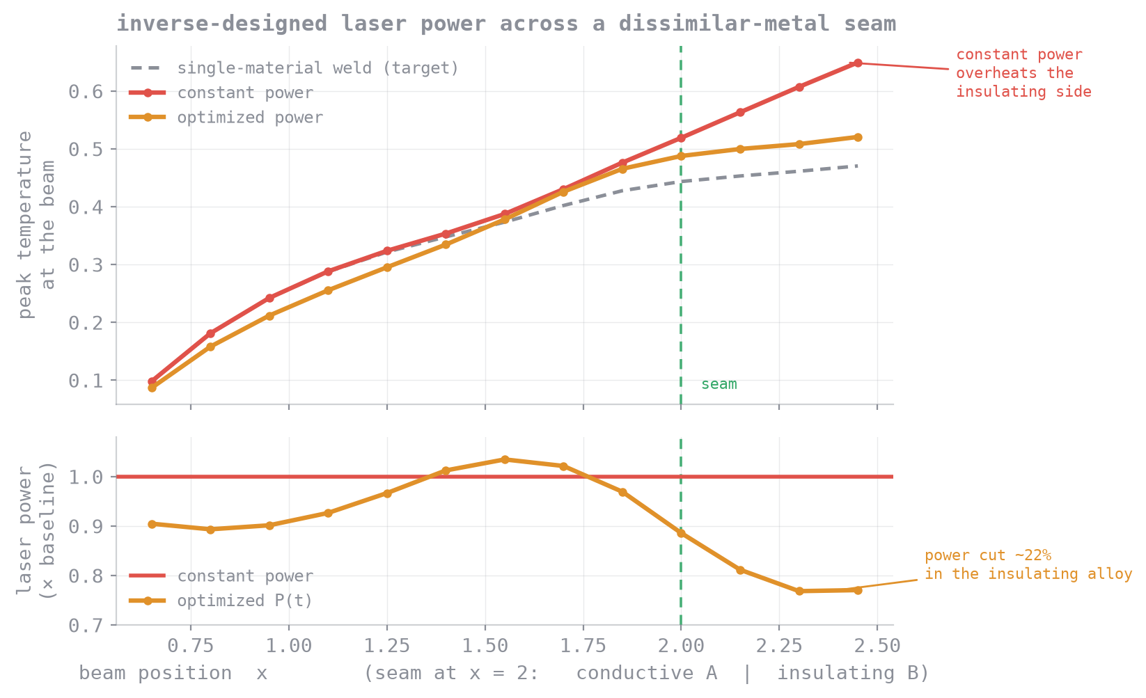
The schedule it discovers is interpretable, which matters: keep roughly full power through the conductive alloy, then drop to about 0.78× as the beam crosses into the insulating side.
Honest scope
This is a proof of concept of the control problem, run on a deliberately coarse mesh with a broadened heat source so the gradient loop stays cheap, not a production weld schedule. The point is narrower and, I think, more useful: the same model that simulates the weld can be turned around and asked to design the process, and that is the real reason to write the physics this way.
The full derivations, validation against the analytic Rosenthal solution, and the interactive version with the solved melt pool are elsewhere:
- The interactive write-up, with the melt pool animation you can orbit and scrub through time.
- Working paper (PDF), derivations, the weak form, and the practical envelope of the differentiable FEM.